Drift and Distance: When Is Score Centering Enough in Async RL?
1UC Berkeley 2Paper Instruments *Equal contribution
In asynchronous RL for LLMs, the sampler generates responses while the trainer updates the policy. The trainer therefore learns from an older policy’s data, creating a gap called staleness. Even without staleness, the two sides can differ. Setup bugs in temperature, top-p, top-k, MoE routing, or tokenization can break training but are easy to fix. Yet different kernels and lower-precision sampling always leave a small mismatch (Fang & Khazi, 2025; Yao et al., 2025).
Score centering (SC) removes the most harmful error that staleness and mismatch cause, a systematic push we call drift (Marek & Ryabinin, 2026). Do we need anything beyond SC? The SC paper pairs SC with truncated importance sampling (TIS) and trains stably. Zhang (2026) finds that the same combination collapses and adds a KL penalty that decays with staleness, while Thinking Machines' StableReinforce pairs SC with a constant KL penalty. The question we ask is, why does the same recipe work in one setup and fail in another?
To find out, we test SC with and without common corrections, such as importance sampling and a KL penalty, while varying staleness, batch size, and learning rate.
Our findings
- SC removes the most harmful error. Without it, training collapses with or without importance sampling, for different reasons, while SC alone trains to the end.
- After SC, what matters is distance, and part of it is learning itself. The remaining risk is how far the trainer moves from the sampler before fresh data arrives. We call this distance and measure it with their KL, which has a noise part and a signal part. A larger batch averages away the noise. The signal part is learning, which piles up on old data, so less staleness or a lower learning rate shrinks it.
- Extra additions to SC help less than expected. In our small-batch, high-staleness settings, truncated importance sampling keeps the trainer somewhat closer to the sampler but does not prevent collapse. A KL penalty prevents collapse, but at best it matches simply lowering the learning rate. With the default penalty used in Thinking Machines' Tinker, a 4B model barely learns.
1. Background and setup
This section introduces the two errors of off-policy data and the corrections that target them, then describes how we test when SC alone is enough.
1.1 Two errors of off-policy data
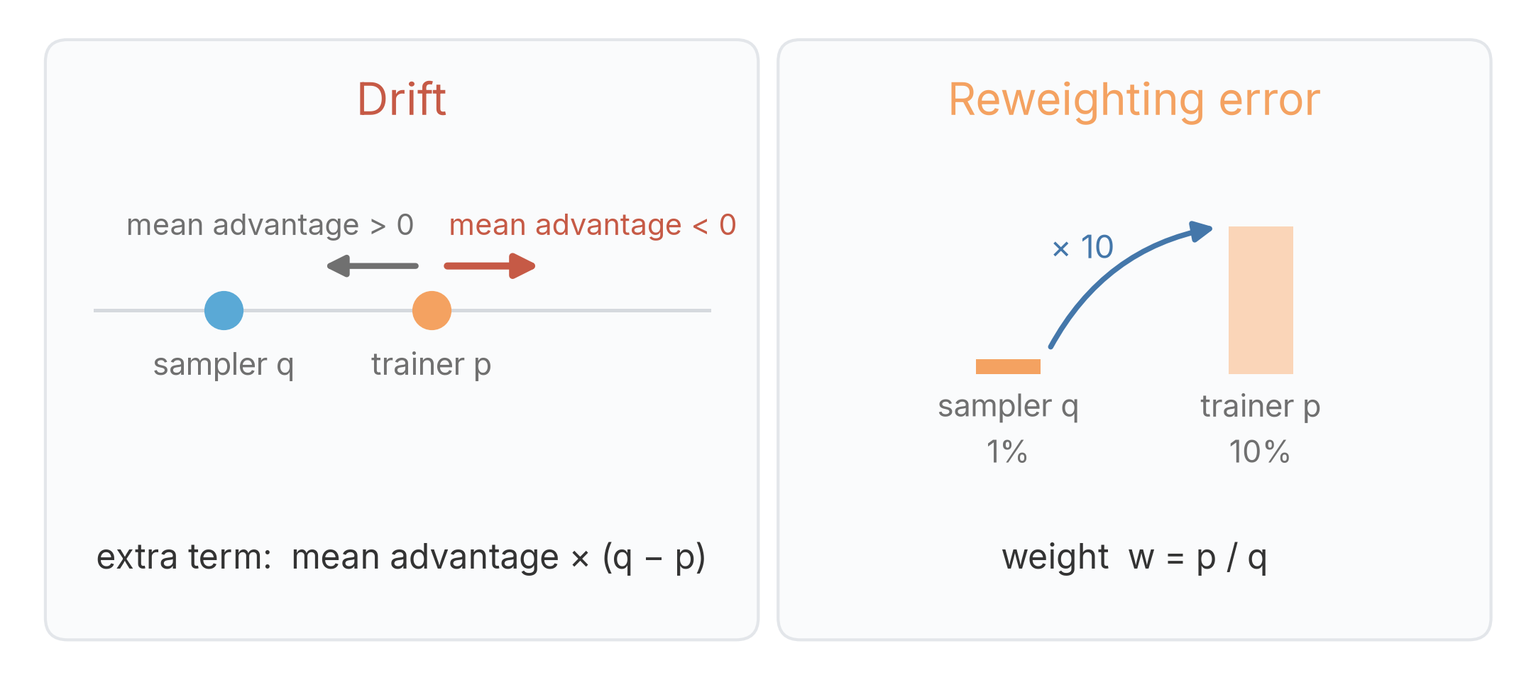
Standard policy gradient assumes that tokens are sampled from the active trainer \(p\) (\(\mathbb{E}_{x \sim p}[A \nabla \log p(x)]\), where \(A\) is token \(x\)'s advantage). In practice, rollouts originate from a sampler \(q\) that differs from \(p\) owing to staleness or setup mismatches. Consequently, the trainer evaluates \(\mathbb{E}_{x \sim q}[A \nabla \log p(x)]\), making the optimization off-policy and inducing two types of errors (Figure 1; Marek & Ryabinin, 2026; Zhang, 2026).
Drift. Under on-policy training, the expected policy gradient contains only the learning signal: it raises the probability of high-advantage tokens. When the data comes from the sampler instead, the expected gradient picks up an extra term that does not depend on which token is better. Under a softmax parameterization, this term points along \(q - p\), scaled by the mean advantage at the prefix.
Reweighting error. The sampler draws tokens from its own distribution, but the trainer needs feedback weighted by its own. If the trainer assigns 10% to a token the sampler assigns 1%, it appears 10× less often than the trainer needs. Weighting it by 10 restores the balance.
Derivation of drift and reweighting error
Fix a prefix and write the trainer's policy as a softmax over logits \(z\). With respect to the logits, \(\nabla_z \log p(x) = e_x - p\), where \(e_x\) is the one-hot vector of token \(x\). We work with logit gradients because they are easy to read. The parameter gradient \(\nabla \log p\) used elsewhere differs only by the chain rule through the logits.
Drift. On-policy, the score averages to zero, \(\mathbb{E}_{x\sim p}[\nabla_z \log p(x)] = p - p = 0\), so the expected gradient \(\mathbb{E}_p[A\nabla_z \log p]\) only says which tokens are better than average. When the data comes from the sampler \(q\), we split each advantage into the mean advantage at the prefix, \(\bar A = \mathbb{E}_q[A]\), and the rest:
\[ \mathbb{E}_{x\sim q}\big[A\,\nabla_z \log p(x)\big] = \underbrace{\mathbb{E}_{x\sim q}\big[(A-\bar A)\,e_x\big]}_{\text{learning signal}} \;+\; \underbrace{\bar A\,(q-p)}_{\text{drift}}. \]
The second term does not depend on which token is better. It points from \(p\) toward \(q\) and is scaled by \(\bar A\), so the trainer is nudged toward the sampler when the mean advantage at the prefix is positive (\(\bar A > 0\)) and away from it when it is negative (\(\bar A < 0\)). Whether this compounds depends on the sampler. A pull toward a fixed, exact sampler, as within a rollout, closes the gap. A pull toward a biased copy of the trainer that is synced every step, as with an fp8 sampler, never settles: each sync gives the target a fresh bias, so the bias accumulates instead of converging (Marek & Ryabinin, 2026). A push away from a fixed sampler grows with \(q - p\), so the further the trainer has moved, the harder it is pushed. Score centering subtracts \(\mathbb{E}_q[\nabla_z \log p] = q - p\) from every score, which removes exactly this term.
Reweighting error. The trainer wants \(\mathbb{E}_{x\sim p}[A\nabla \log p(x)]\), but its data comes from \(q\). Importance sampling rewrites this target as an average over the sampler's data:
\[ \mathbb{E}_{x\sim p}\big[A\,\nabla \log p(x)\big] = \mathbb{E}_{x\sim q}\Big[\tfrac{p(x)}{q(x)}\,A\,\nabla \log p(x)\Big]. \]
Without the weight \(w = p/q\), each token counts with the sampler's frequency instead of the trainer's, and this error grows with the KL between the two policies. With the weight, the average is correct, but its variance grows with \(\mathbb{E}_q[w^2]\).
1.2 Three corrections
Three corrections are in common use. Score centering targets drift, importance sampling targets reweighting error, and a KL penalty keeps the trainer near the sampler.
- Score centering (SC) removes drift without introducing weights. It recenters each token’s gradient around its average under the sampler. That average is what drift adds, so subtracting it cancels drift. The reweighting error remains.
- Importance sampling (IS) corrects reweighting error by weighting each token by \(w = p/q\), which makes the average match the on-policy one, \(\mathbb{E}_{x\sim q}[w\,A\,\nabla\log p] = \mathbb{E}_{x\sim p}[A\,\nabla\log p]\). The weights add variance, which grows with \(\mathbb{E}_q[w^2]\) and is driven by a few extreme weights. Truncated importance sampling (TIS) truncates the weights at a ceiling \(C\) (Yao et al., 2025).
- A KL penalty pulls the trainer back toward the sampler with strength \(\beta\).
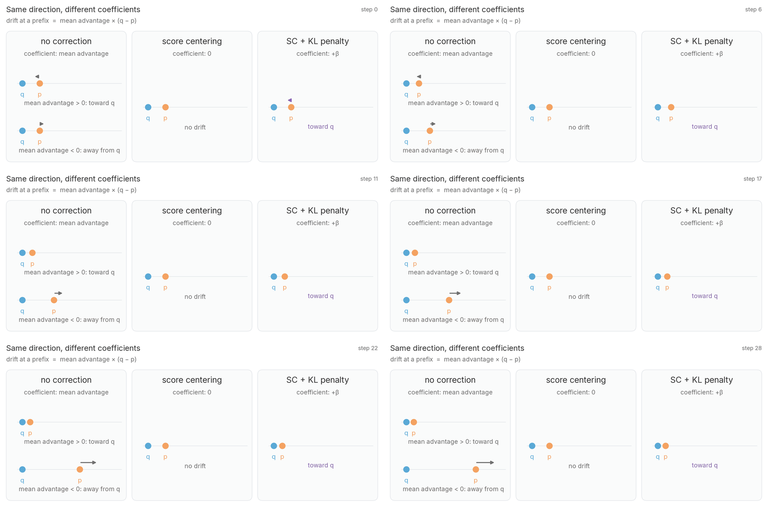
Figure 2 shows the coefficient each correction puts on the drift term. Without correction, it is the mean advantage at the prefix and can have either sign. A positive coefficient pulls the trainer toward the sampler. When the sampler is a biased copy of the trainer, as with an fp8 sampler, every weight sync gives it a fresh bias, so the pull never settles and the error accumulates (Marek & Ryabinin, 2026). A negative coefficient pushes the trainer away, harder the further it has gone. SC sets the coefficient to zero, and SC plus a KL penalty sets it to \(+\beta\), which always pulls toward the sampler.
1.3 When is SC enough?
SC removes drift but leaves the reweighting error, which grows with how far the trainer moves from the sampler before fresh data arrives (Zhang, 2026). We call this distance and measure it with the KL between the two. To find when SC alone stays stable, we vary batch size and staleness, which differ most between the setups we started from, and test whether importance sampling or a KL penalty helps when it does not.
1.4 Experimental setup
We train Qwen3.5-0.8B-Base on GSM8K for 640 steps in SkyRL with vLLM sampling, and check the main results on Qwen3.5-4B-Base. Each optimizer step uses 32 to 1,024 responses (16 to 128 for 4B). The fixed settings are listed in the configuration below.
Training configuration
| Setting | Value |
|---|---|
| Sampling | 8 responses per problem, temperature 1.0, no top-p or top-k, up to 4,096 tokens |
| Advantage | reward minus the group mean, without std scaling, as in Dr. GRPO (Liu et al., 2025) |
| Learning rate | 0.03 for 0.8B unless noted, 0.033 for 4B |
| Score centering | the sampler’s top-32 log-probabilities, returned by vLLM |
| Truncated IS | ceiling \(C = 2\) |
| 4B data and evaluation | DAPO-Math-17k, evaluated on AIME 2024 and 2025 (16 samples per problem) and MATH-500 |
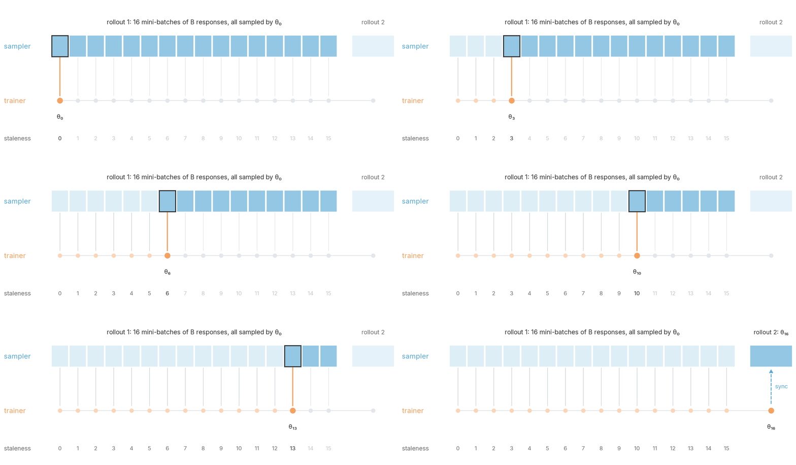
Controlling staleness. We emulate staleness in a synchronous loop (Figure 3). Each rollout, the responses sampled between two weight syncs, is split into \(N\) mini-batches of \(B\) responses (the batch size), with one SGD step on each. The last mini-batch is \(N - 1\) steps stale, and we name each setting by this maximum staleness, so \(N = 64\) is staleness 63 and \(N = 1\) has no staleness, which we call on-policy. The corrections use the sampler's recorded log-probabilities, so they also see the train-inference mismatch of real async RL.
Optimizer. We use plain SGD rather than Adam. Adam normalizes each parameter’s update, so changing the batch size would change the effective step size as well as the noise. With SGD and the loss averaged over the batch, only the noise changes.
What we measure. We plot the training reward of each rollout at the step it was sampled. Gray dashed curves are on-policy runs with the same batch size and learning rate. A collapse (×) is the first rollout with reward below 1%, and end reward averages the last three rollouts. All full 0.8B runs take 640 steps, so a larger batch also sees more samples.
2. SC stabilizes training, but not always
We first test SC and importance sampling side by side in one setting, then make the batch larger, and then make the data older and the batch smaller.
2.1 Removing drift: SC and importance sampling, each on and off
We start with batch 64 and a maximum staleness of 15. Figure 4 runs three strategies, no importance sampling (no IS), untruncated importance sampling (vanilla IS), and truncated importance sampling (TIS, ceiling \(C = 2\)), each with and without SC.
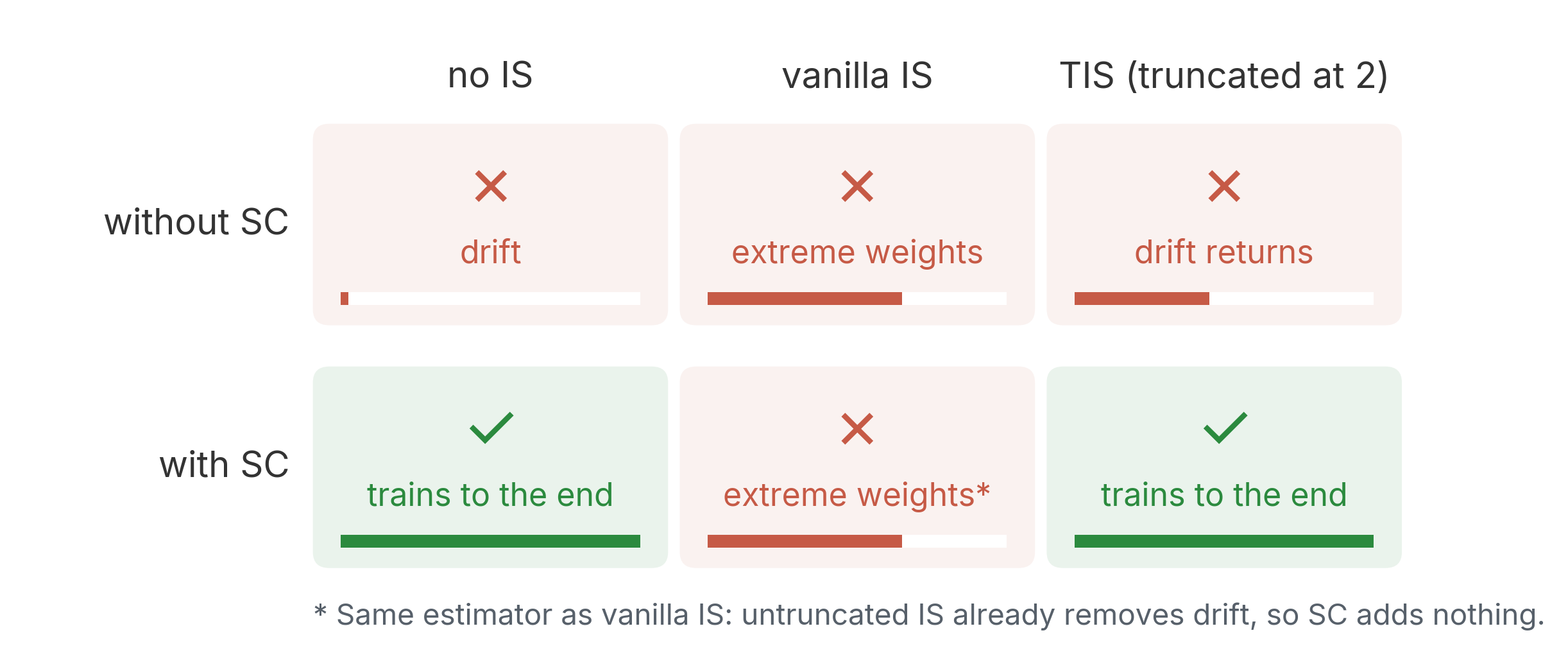
Without SC, all three runs collapse. No IS keeps all of the drift, TIS leaves the drift on the tokens it truncates, and vanilla IS fails from extreme weights instead (Section 4.2).
With SC, SC alone and SC + TIS train to the end. SC + vanilla IS, starred in Figure 4, collapses exactly like vanilla IS, from extreme weights rather than drift (Section 4.2). In this setting, SC alone is enough.
How the six runs differ
All six can be written in a single formula. For each token, the update direction is:
\[ \hat g = A \Big( w(x)\,\nabla\log p(x) \;-\; \mathbb{E}_{x'\sim q}\big[w(x')\,\nabla\log p(x')\big] \Big), \]
where \(x\) is the sampled token, \(A\) is its advantage, and the expectation runs over all candidate tokens at that position under the sampler \(q\). The weight \(w\) depends on the IS variant: \(w = 1\) for no IS, \(w = p(x)/q(x)\) for vanilla IS (the ratio \(\pi_{\text{train}}/\pi_{\text{rollout}}\)), and \(w = \min(p(x)/q(x),\, C)\) for TIS. The second term inside the parentheses is SC, the sampler average that cancels drift. Without SC, only the first term remains.
Vanilla IS removes drift in expectation. With \(w = p/q\), \(\mathbb{E}_q[w\nabla\log p] = \mathbb{E}_p[\nabla\log p] = 0\), so the SC term is already zero. This is why the starred run in Figure 4 matches vanilla IS.
2.2 Large batches: SC alone keeps up with on-policy training
Batch 64 was small enough for vanilla IS to collapse. We now raise the batch to 512 at the same staleness and ask whether that keeps all three methods stable (Figure 5).
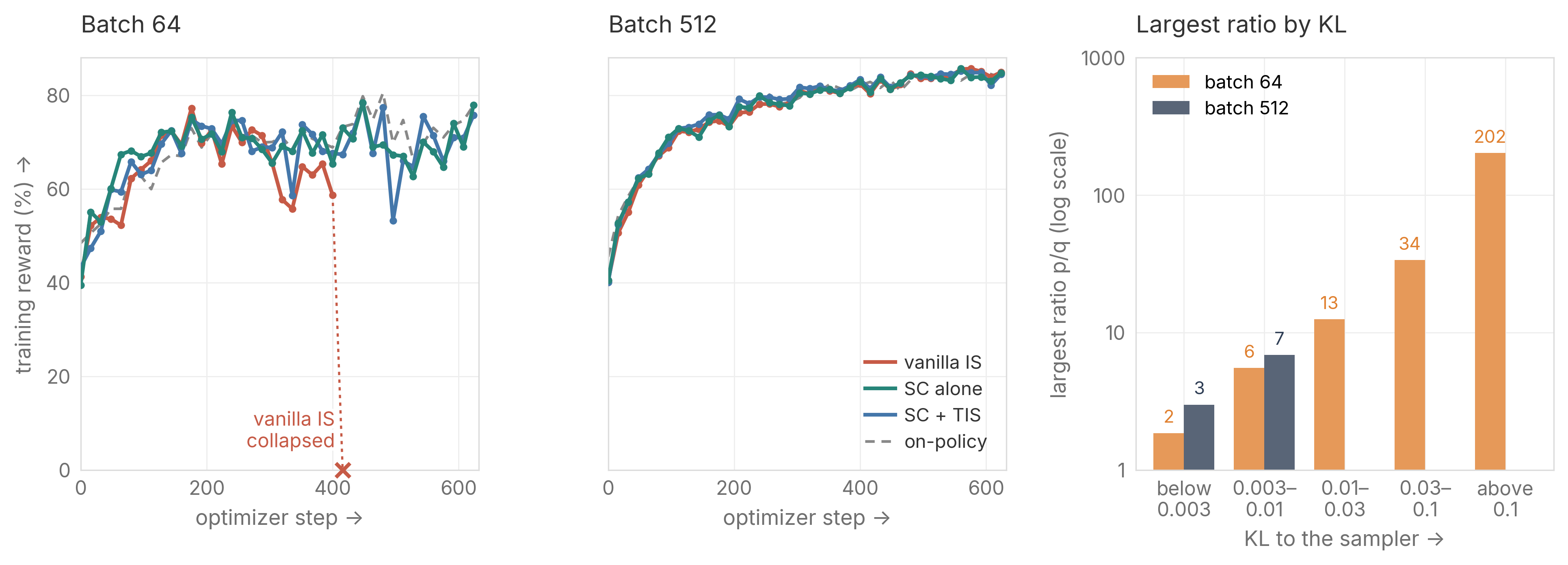
The left two panels of Figure 5 show that a larger batch stabilizes all three methods. At batch 512, they all keep up with on-policy to the end, while at batch 64 the curves are noisy and vanilla IS collapses. The next subsection shows the same pattern on 4B at batch 128.
The larger batch works by shrinking the distance. With less noise per step, the trainer does not move away from the sampler by chance. An 8× larger batch lowers the median KL about 8×, and truncation almost never triggers. Section 3 explains why the drop is so close to 8×.
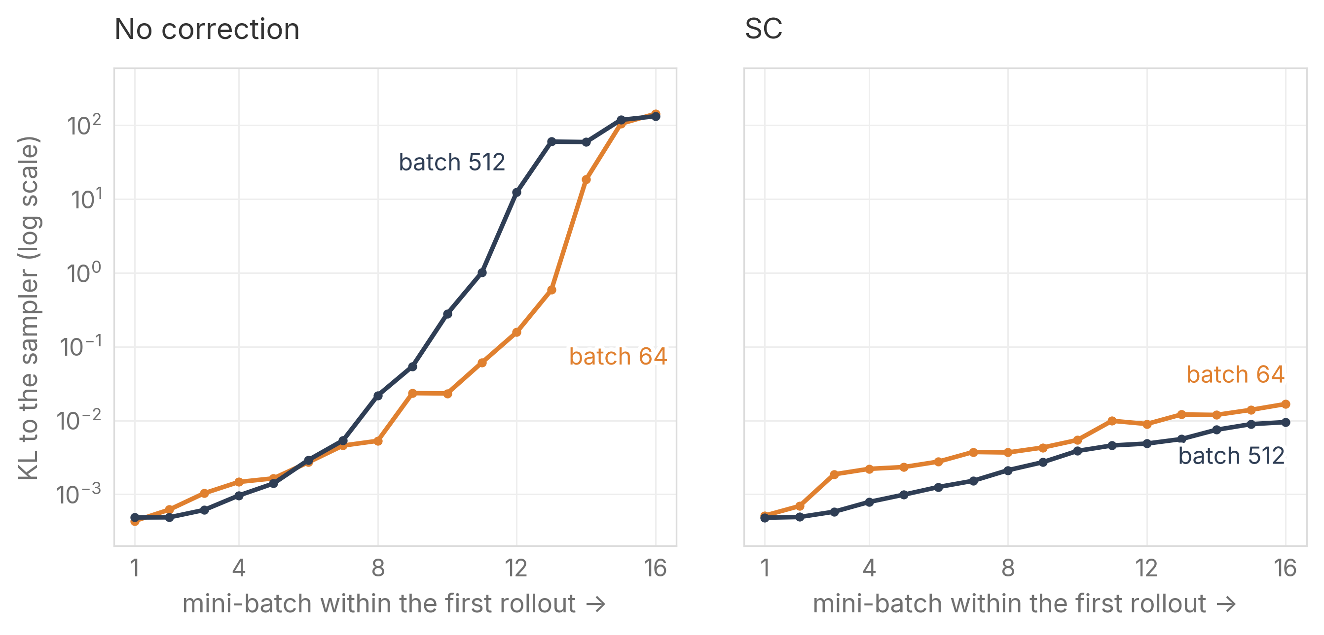
Figure 6 shows that a larger batch helps only once drift is removed. Without correction, the KL runs away within the first rollout at batch 512 just as at batch 64. Drift pushes every step in the same direction, and a larger batch averages away only random noise. With SC, the KL stays small at both, and batch 512 ends the rollout at about half the KL of batch 64.
2.3 High staleness and small batches: SC alone can break
Next we move to the opposite regime, with older data and smaller batches. At high staleness the trainer takes many steps on the same data and moves far from the sampler, and that distance is what can break SC. We run SC alone at staleness 63, so each rollout feeds 64 mini-batches, with batches of 32, 64, and 512.
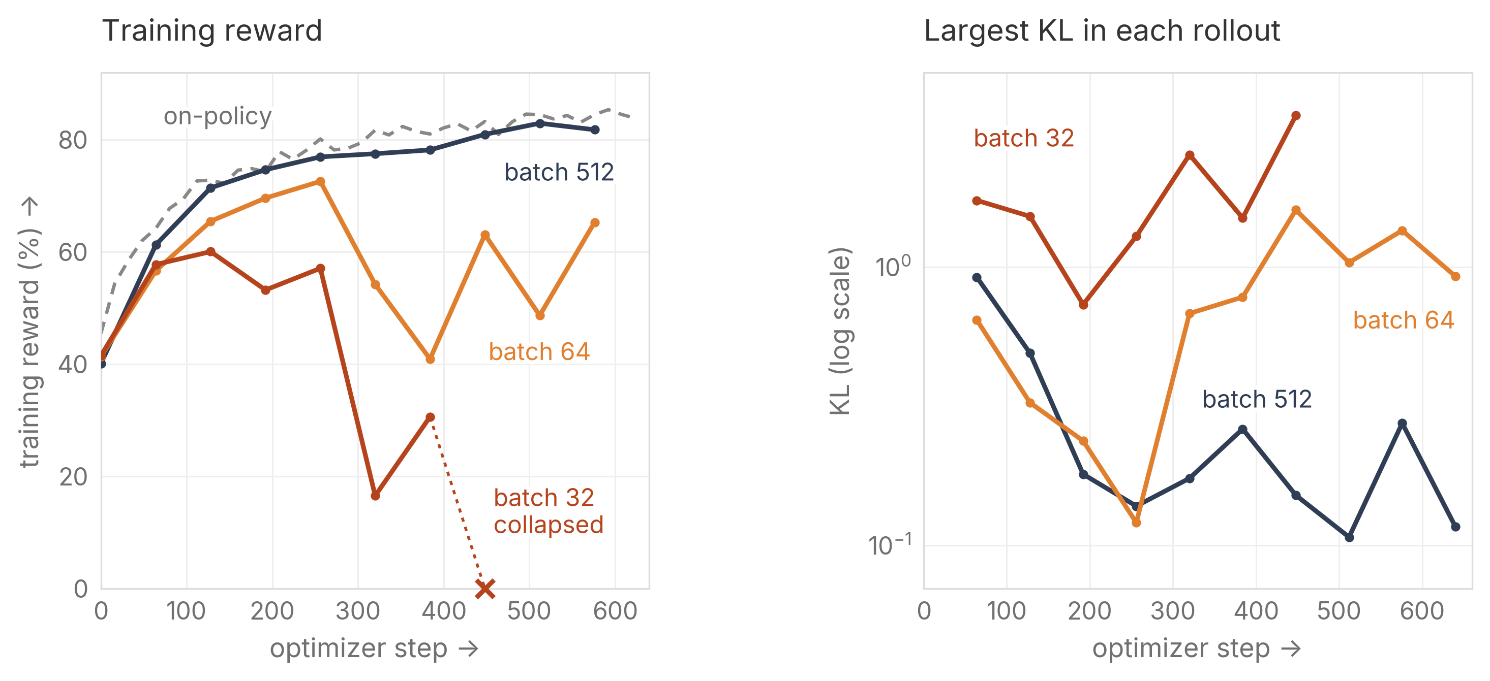
The left panel of Figure 7 shows that SC alone keeps up with on-policy at batch 512 but breaks at smaller batches. Batch 32 collapses at step 448. Batch 64 trains to the end but finishes 14 points below its best. In the right panel, the smaller the batch, the higher the largest KL in each rollout. The same holds on a larger model and harder data: 4B on DAPO-Math-17k at staleness 15, where we also compare the three methods.
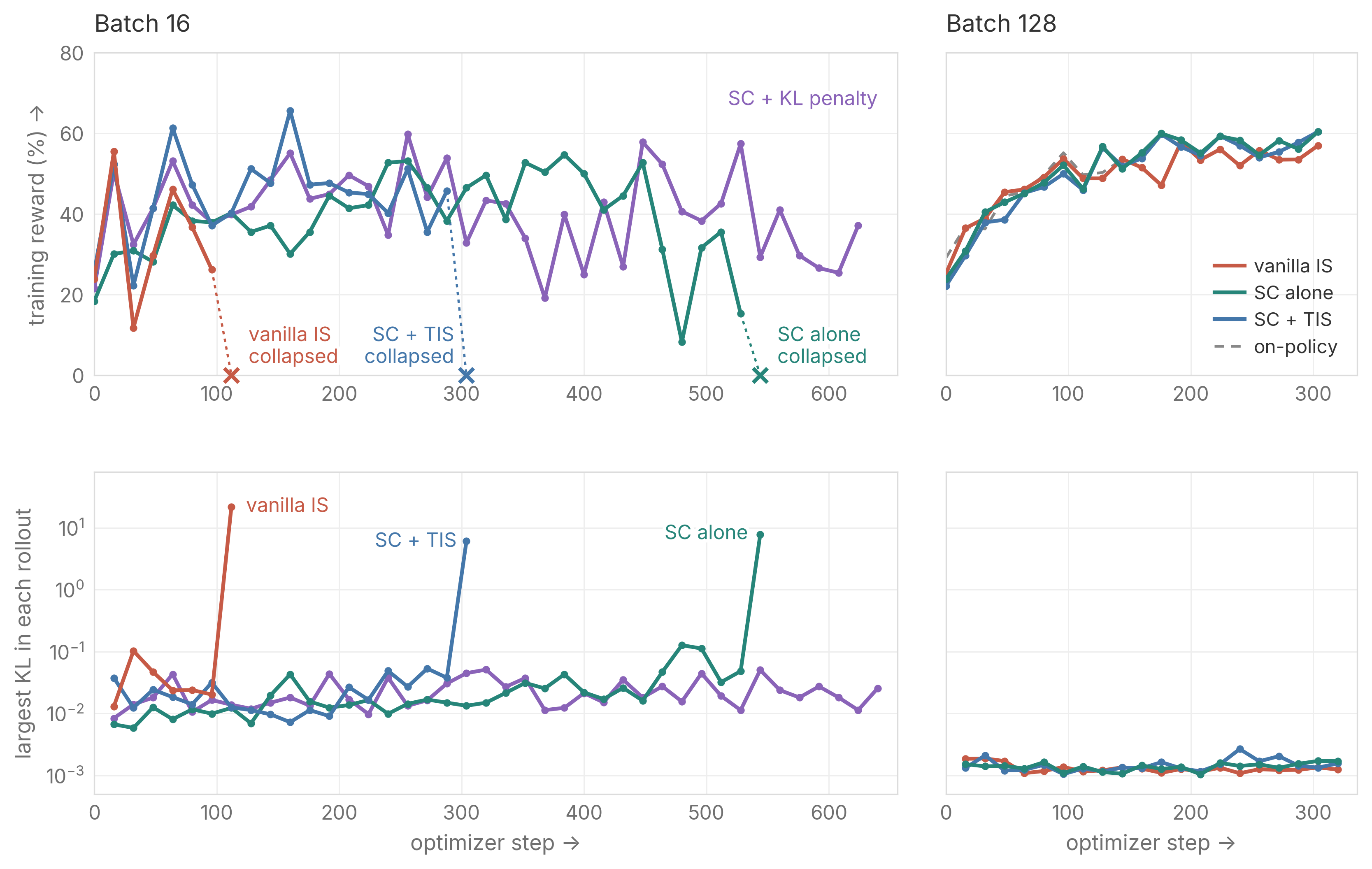
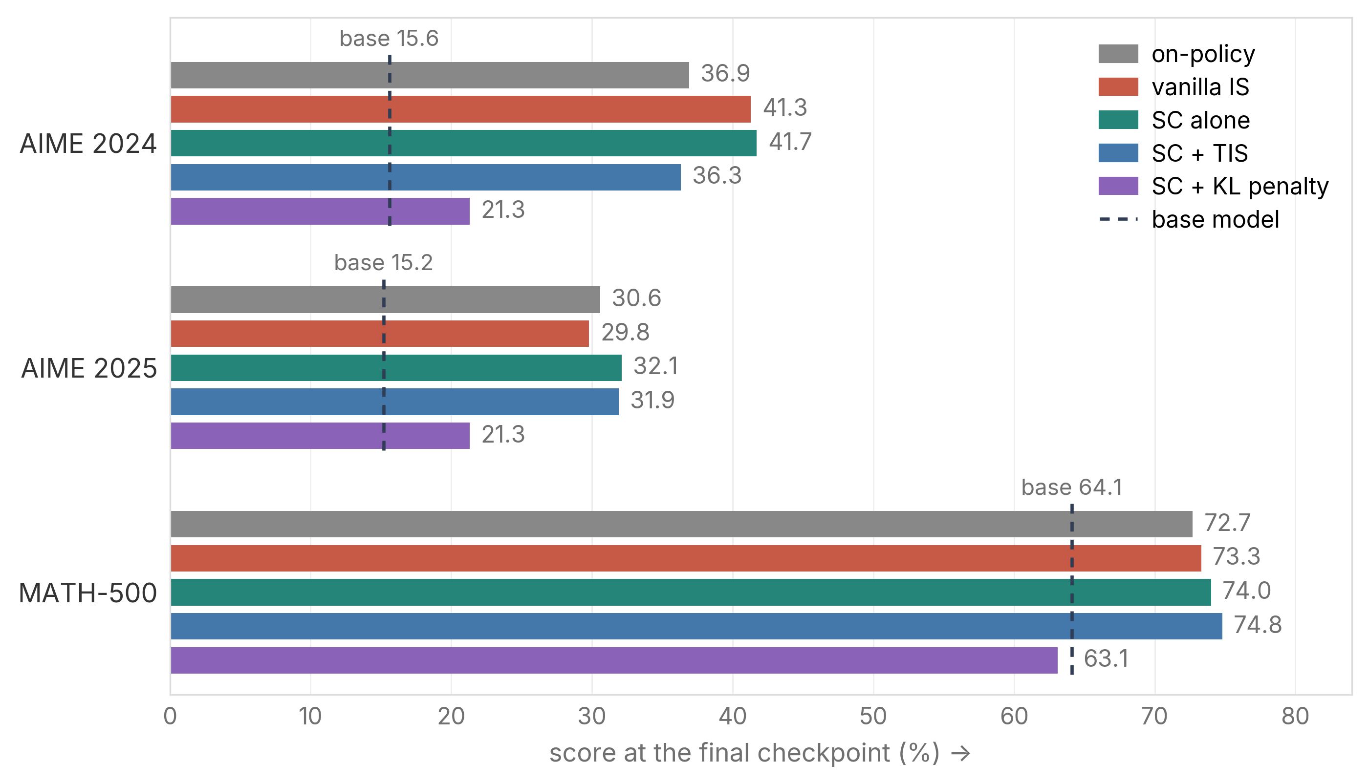
The 4B runs in Figure 8 fail the same way at small batch. At batch 16, all three methods collapse, and each collapse starts with a sudden spike in the KL to the sampler. At batch 128, all three keep up with on-policy and roughly double the base model’s AIME scores. The differences among them are within sampling error (see the evaluation below). In both models, every failure comes with a large KL to the sampler, and a larger batch keeps that KL small. Why does the batch matter so much, and does it always help?
4B evaluation
3. Why SC fails: noise and learning in the distance
To understand why the batch matters so much, we split the distance into two parts. Gradient noise moves the trainer in a random direction at each step, and a larger batch averages it away. The learning signal moves it in the same direction at every step, so on stale data it keeps adding up. This accumulation is simply the learning process at work, staying present at any batch size.
Definition. We measure distance with the per-token KL, \(\mathrm{KL}(q \,\|\, p_k)\), between the sampler's policy \(q\) and the trainer's policy \(p_k\) after \(k\) steps of a rollout. We estimate it on the sampled tokens as the mean of \(w - 1 - \log w\), with \(w = p/q\) (Schulman, 2020). It starts near zero and grows with each step.
Signal and noise. Each step's gradient estimate is \(\hat g_i = g + \varepsilon_i\). The signal \(g = \mathbb{E}[\hat g_i]\) is the direction all batches agree on. The noise \(\varepsilon_i\) is specific to the current batch, with zero mean and variance proportional to \(1/B\). Each SGD step moves the parameters by \(-\eta\,\hat g_i\), so after \(k\) steps they have moved by
\[ \theta_k - \theta_0 = -\eta\Big(\underbrace{k\,g}_{\text{signal: grows like } k} + \underbrace{\varepsilon_1 + \cdots + \varepsilon_k}_{\text{noise: grows like } \sqrt{k}}\Big). \]
The signal adds up in one direction, so it grows like \(k\). The noise partly cancels across steps, so it grows only like \(\sqrt{k}\). The KL grows roughly with the square of this displacement, so it splits into two terms:
\[ \mathrm{KL}_k \;\approx\; c_{\text{noise}}\,\frac{\eta^2 k}{B} \;+\; c_{\text{signal}}\,\eta^2 k^2, \]
where \(c_{\text{noise}}\) is set by the gradient variance and \(c_{\text{signal}}\) by the size of the signal.
Derivation of the two terms
Near the sampler, the KL is a quadratic form of the displacement, \(\mathrm{KL} \approx \tfrac{1}{2}\Delta\theta^\top F \Delta\theta\), where \(F\) is the Fisher information matrix and measures how sensitive the policy is along each direction. We treat \(g\) and \(F\) as constant within a rollout.
- Step \(i\) adds \(-\eta(g + \varepsilon_i)\). Summing \(k\) steps gives the displacement above.
- Substituting it into the quadratic form gives \(\tfrac{1}{2}\eta^2 (kg + \textstyle\sum_i \varepsilon_i)^\top F (kg + \textstyle\sum_i \varepsilon_i)\).
- The signal–signal part is \(\tfrac{1}{2}\eta^2 k^2\, g^\top F g = c_{\text{signal}}\,\eta^2 k^2\), so \(c_{\text{signal}} = \tfrac{1}{2} g^\top F g\) is the squared length of the signal, weighted by sensitivity.
- Each cross term contains a single \(\varepsilon_i\), whose mean is zero, so it vanishes in expectation.
- In the noise–noise part, terms with \(i \ne j\) vanish because different mini-batches are independent. Each of the \(k\) terms with \(i = j\) has expectation \(\tfrac{1}{2}\mathrm{tr}(F\Sigma)/B\), where \(\Sigma\) is the gradient covariance of a single response, so a mini-batch of \(B\) responses has covariance \(\Sigma/B\). Together they give \(c_{\text{noise}}\,\eta^2 k/B\), with \(c_{\text{noise}} = \tfrac{1}{2}\mathrm{tr}(F\Sigma)\).
What each setting does. Batch size, learning rate, and staleness act on the two terms differently, and each has its own cost:
| Setting | Noise term | Signal term | Cost |
|---|---|---|---|
| Larger batch \(B\) | ✅ shrinks as \(1/B\) | ❌ unchanged | more samples per step |
| Lower learning rate \(\eta\) | ✅ shrinks as \(\eta^2\) | ✅ shrinks as \(\eta^2\) | less learning per step |
| Less staleness \(k\) | ✅ shrinks as \(k\) | ✅ shrinks as \(k^2\) | more frequent sampler syncs |
On the stalest mini-batches, the signal term dominates, so less staleness helps most and a larger batch least. The two terms are also not equally useful. Distance from noise brings no learning, while distance from the signal comes from learning itself. A larger batch removes only the first, and the other two settings shrink both.
Testing the formula. The table above says a larger batch shrinks only the noise term, so we can test it by changing the batch alone. If the KL were all noise, an 8× larger batch would cut it 8×. If it were all signal, the larger batch would not change it. We run one rollout at batch 128 and one at batch 1024, and Figure 10 plots the ratio of their KLs at every step.
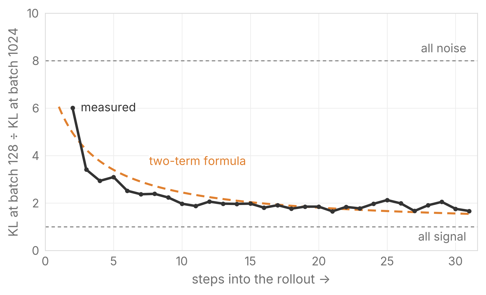
The ratio starts near 6, so while the data is still fresh, most of the KL is noise. By the last step it falls below 2, because the signal has piled up and a larger batch cannot remove it. The two-term formula, fitted on other runs, predicts the same decline (orange dashed curve). A larger batch therefore helps least on the stalest mini-batches, where the KL is largest and SC breaks.
4. What helps when SC fails
SC alone breaks once the trainer moves far from the sampler, that is, once the largest KL in a rollout grows large. We compare three ways to rescue it: changing the settings that set this distance, adding importance weights, and adding a KL penalty that pulls the trainer back.
4.1 Training settings: control the distance at the source
The most direct fix is to change the settings that set the distance. Starting from a run where SC alone breaks, Figure 11 changes one setting at a time. Each change keeps the largest KL in every rollout far below that of the starting run (bottom row), and SC alone then trains to the end.
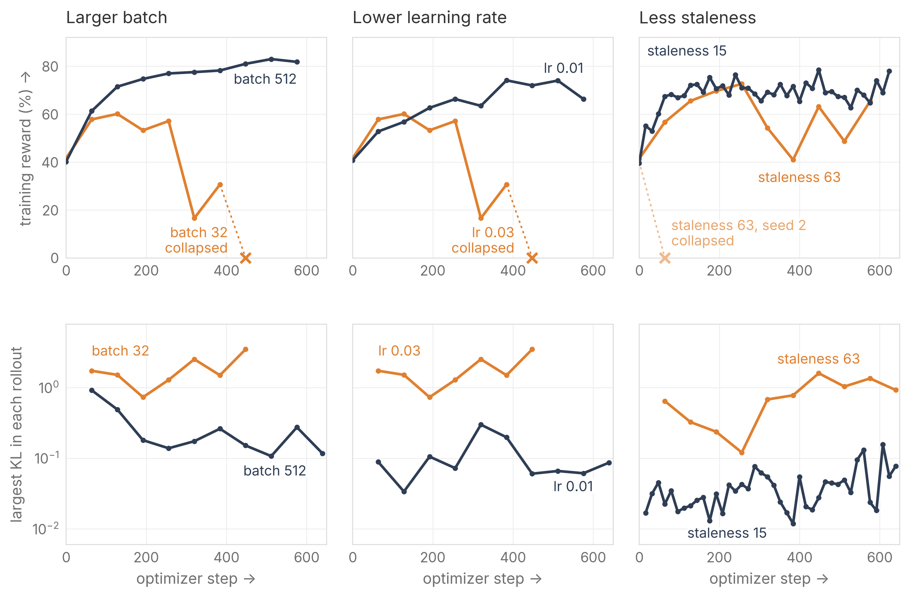
A larger batch, a lower learning rate, and less staleness each rescue SC, by different amounts:
- Larger batch. In the first rollout, going from batch 32 to 512 only halves the largest KL (1.7 to 0.9): training has just begun, the learning signal is strong, and about half of the KL comes from it. Later in training the signal weakens and most of the KL is noise, so the same change cuts it about 9× (1.6 to 0.18).
- Lower learning rate. Cutting it to a third lowers the KL by more than an order of magnitude, whatever the KL is made of.
- Less staleness. It is the main fix for very old data. Going from 63 to 15 at batch 64 cuts the KL by more than the ratio squared (about 18×), and SC trains to the end (Figure 11, right).
The two-term formula assumes that the gradient and the curvature stay fixed within a rollout, so it predicts these reductions well while the trainer stays close to the sampler. After many steps on the same data at learning rate 0.03, the KL grows faster than the formula allows, so a lower learning rate or less staleness helps even more than predicted.
| KL ratio in the first rollout at staleness 63 (formula in parentheses) | Step 4 | Step 16 | Step 63 |
|---|---|---|---|
| Batch 32 / batch 512 | 7.0× (9.5×) | 3.8× (4.7×) | 2.1× (2.1×) |
| Learning rate 0.03 / 0.01 | 8.3× (9×) | 16× (9×) | 33× (9×) |
Why the KL grows faster than the formula
The formula assumes that the gradient stays the same throughout a rollout. With SC alone at staleness 63 and batch 512 it does not: the KL added per step keeps speeding up. Most of the speed-up comes from the learning signal pushing down tokens that are already below the sampler. Three variants of that run, two seeds each, show this. At the end of the first rollout, SC alone reaches a KL of 0.6–1.1.
- Scaling the terms with negative advantage by \(\min(1, w)\) brings it to 0.06, about 14× lower.
- Fixing the size of each step brings it to 0.33, about 2.6× lower.
- Flipping the sign of each advantage at random, which removes the learning signal, brings it to 0.004, about 200× lower.
This is also why a lower learning rate helps more than the formula predicts (table above).
4.2 Importance weights: not always safer
Another option is to add importance weights on top of SC, to correct the reweighting error that SC leaves. With full weights, SC has nothing left to do: vanilla IS already removes drift in expectation, and SC + vanilla IS is the same estimator as vanilla IS (the starred run in Figure 4). Weights on top of SC are therefore truncated, as in TIS, and SC centers with the same truncated weights so that drift stays out. TIS does two things: it truncates the large weights and keeps the small ones.
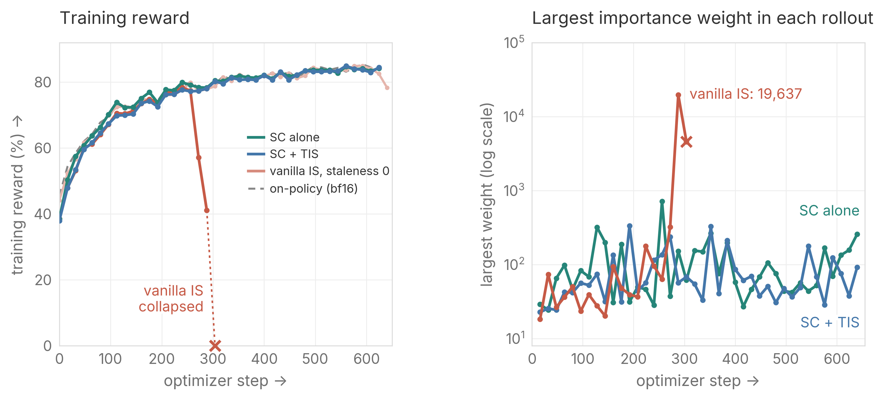
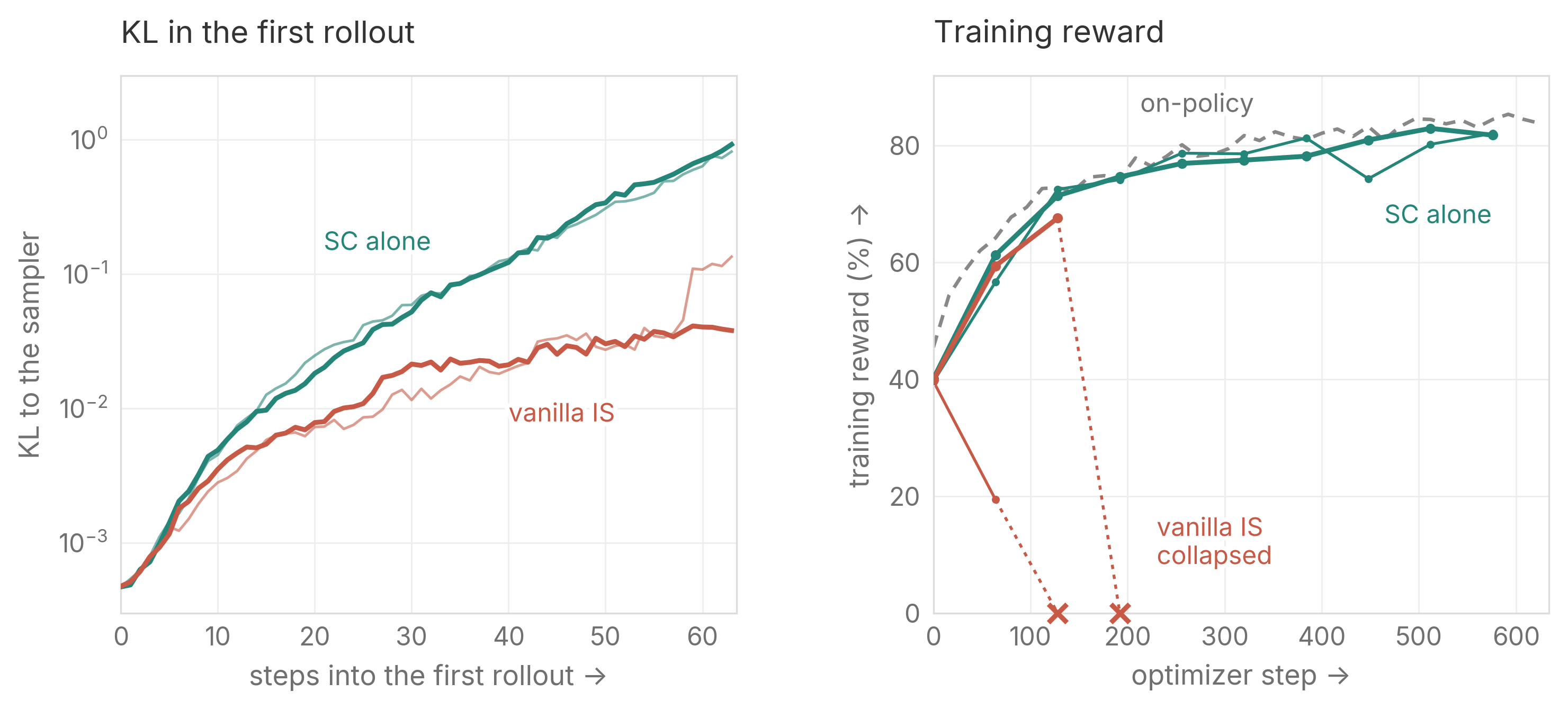
Why truncate the large weights. A token gets a large weight when the trainer gives it much more probability than the sampler did. Untruncated, such weights break training even when the mismatch is small. In Figure 12 the sampler runs in fp8 and the trainer in bf16. With a bf16 sampler in the same setting, vanilla IS trains to the end (Figure 5). The fp8 rounding adds only a small mismatch, yet one weight jumps to nearly 20,000 (right) and vanilla IS collapses, while SC alone and SC + TIS train to the end (left). With older data, vanilla IS collapses even while it stays 10× closer to the sampler than SC alone (Figure 13).
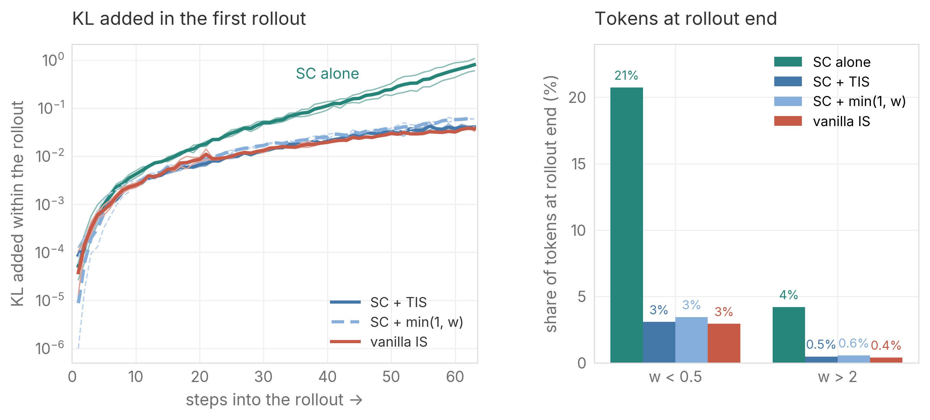
What the small weights keep. IS multiplies each token's update by its weight \(w = p/q\). Once the trainer gives a token less probability than the sampler, \(w < 1\), and every further push on that token shrinks with \(w\). SC does not reweight tokens, so it keeps pushing them down at full strength and they sink further below the sampler. In Figure 14, SC alone ends with 21% of tokens below \(w = 0.5\), against 3% for vanilla IS (right). Adding only this scaling to SC, by multiplying the terms with negative advantage by \(\min(1, w)\), brings the KL down more than tenfold, to where SC + TIS and vanilla IS end (left). This missing scaling is what moves SC alone so far.
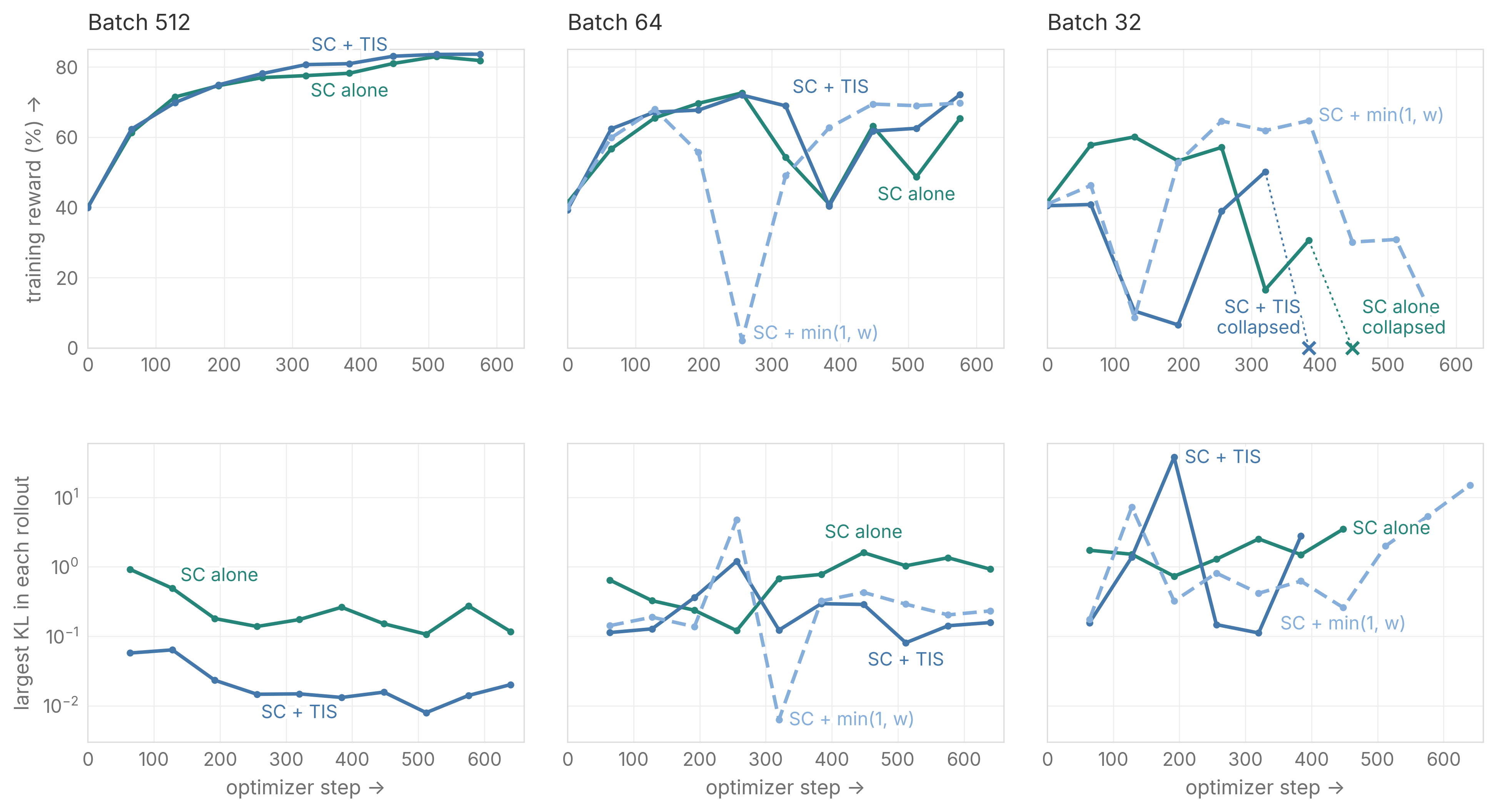
SC + TIS still collapses at small batches. In our settings, truncation removes the failure of large weights and the small weights shrink the KL, yet SC + TIS still collapses at small batches in the same settings as SC alone (Figure 15, and Figure 8 on 4B), and so does SC + \(\min(1, w)\). At large batches SC + TIS trains to the end. The SC paper, with 512 responses per step, finds it ahead of SC alone (Marek & Ryabinin, 2026). In our runs at batch 512, and on 4B at batch 128, it ends level with SC alone.
4.3 A KL penalty: stability at a cost, but worth exploring
The last option is a KL penalty. Instead of changing the source, it adds a pull back toward the sampler that grows with the distance. That pull acts on every move, whether from noise or from learning, so a strong penalty also holds back learning. Can it beat a lower learning rate?
Derivation of how the KL penalty limits distance
Near the sampler, the gradient of \(\beta\,\mathrm{KL}(q \,\|\, p_\theta)\) is about \(\beta F \Delta\theta\), and the displacement follows
\[ \Delta\theta_{k+1} = (I - \eta\beta F)\,\Delta\theta_k \;-\; \eta\,(g + \varepsilon_k). \]
Along a direction of curvature \(\lambda\), each step shrinks the existing displacement by a factor \(1 - \eta\beta\lambda\). After about \(1/(\eta\beta\lambda)\) steps, neither the signal nor the noise term grows any further, so the penalty limits how far the trainer can move within a rollout. It also means that after \(k\) steps, mini-batch \(j\) counts with weight \((1 - \eta\beta\lambda)^{k-j}\), so the older a mini-batch is, the less it counts. A lower learning rate weights every mini-batch equally, and for the same learning signal, equal weights leave the least noise.
Figure 16 compares penalties of different strengths with simply lowering the learning rate, at batch 32 and staleness 63, where SC alone collapses. The measured KL tells us how far to lower it. The largest KL in each rollout is about 1.6 here, against about 0.18 for SC alone at batch 512, which trains to the end. Since the KL grows with the square of the learning rate, closing that ninefold gap takes a third of the step. With the learning rate cut to a third, the largest KL falls about twentyfold, and SC trains to the end.
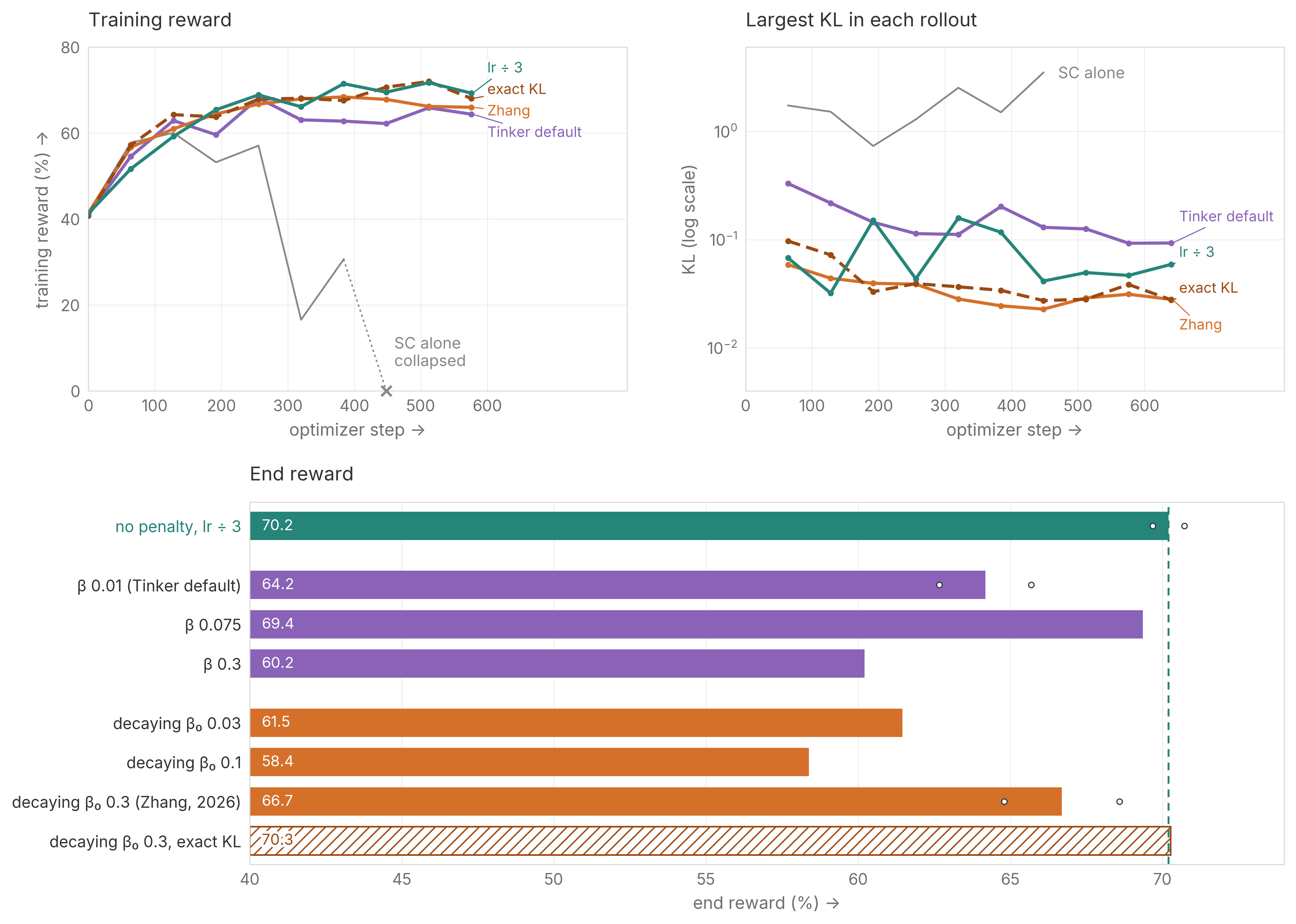
Every penalty stops the collapse, but only a tuned one matches the lower learning rate. Tinker's default (\(\beta = 0.01\)) is too weak. It leaves the KL high and ends 6 points lower. A strong penalty (\(\beta = 0.3\)) keeps the KL lowest, yet ends 10 points lower, because it also holds back learning. Only \(\beta = 0.075\), in between, matches the lower learning rate.
A penalty that decays with token age does no better. We also ran the schedule from Zhang (2026), which weakens the penalty as \(\beta_0/\sqrt{\text{age}}\) (orange in Figure 16). It helps over a constant penalty of the same starting strength, and the best schedule, \(\beta_0 = 0.3\) with the exact KL, only matches the lower learning rate. Zhang (2026) and StableReinforce both estimate the KL from the sampled token alone. With SC, compute the exact KL over the tokens SC already records instead, so it comes almost free. In our runs these are the sampler's top 32, and the exact KL lifts decaying \(\beta_0 = 0.3\) from 66.7 to 70.3.
Why a lower learning rate matches a tuned penalty
Four things favor the learning rate. First, the penalty forgets. Every step it pulls the trainer back toward the sampler, which undoes part of what earlier mini-batches taught, so by the end of a rollout the update reflects mostly the last few mini-batches and rests on fewer samples. A lower learning rate shrinks every step equally and forgets nothing. The KL within a rollout shows this: under the lower learning rate it keeps growing until the last mini-batch, while under a constant penalty it levels off. Second, the learning rate is easy to set. The KL scales with \(\eta^2\), so the measured KL tells you how far to cut, while the right penalty strength depends on curvature and rollout length and has to be found by search. Third, the penalty is only as good as its KL estimate. The one-token estimate, \(\log q - \log p\) on the sampled token, adds noise to every step: with it, decaying \(\beta_0 = 0.3\) ends at 66.7, and with the exact KL over the sampler's top-32 tokens the same schedule ends at 70.3, level with the lower learning rate. Finally, a strong penalty holds back learning too. At \(\beta = 0.3\), the KL stays several times below that of the lower learning rate, and the run ends 10 points lower.
On 4B, the default penalty barely learns. With Tinker’s default penalty on DAPO-Math at batch 16 (purple in Figure 8), SC no longer collapses, but the training reward never trends up. Its final checkpoint scores 21% on AIME, close to the base model and far below the batch-128 runs (Figure 9). The same \(\beta\) that was too weak on 0.8B holds back learning here, so a penalty strength tuned in one setup does not carry over to another.
5. A checklist for async RL
Figure 17 turns our results into a checklist.
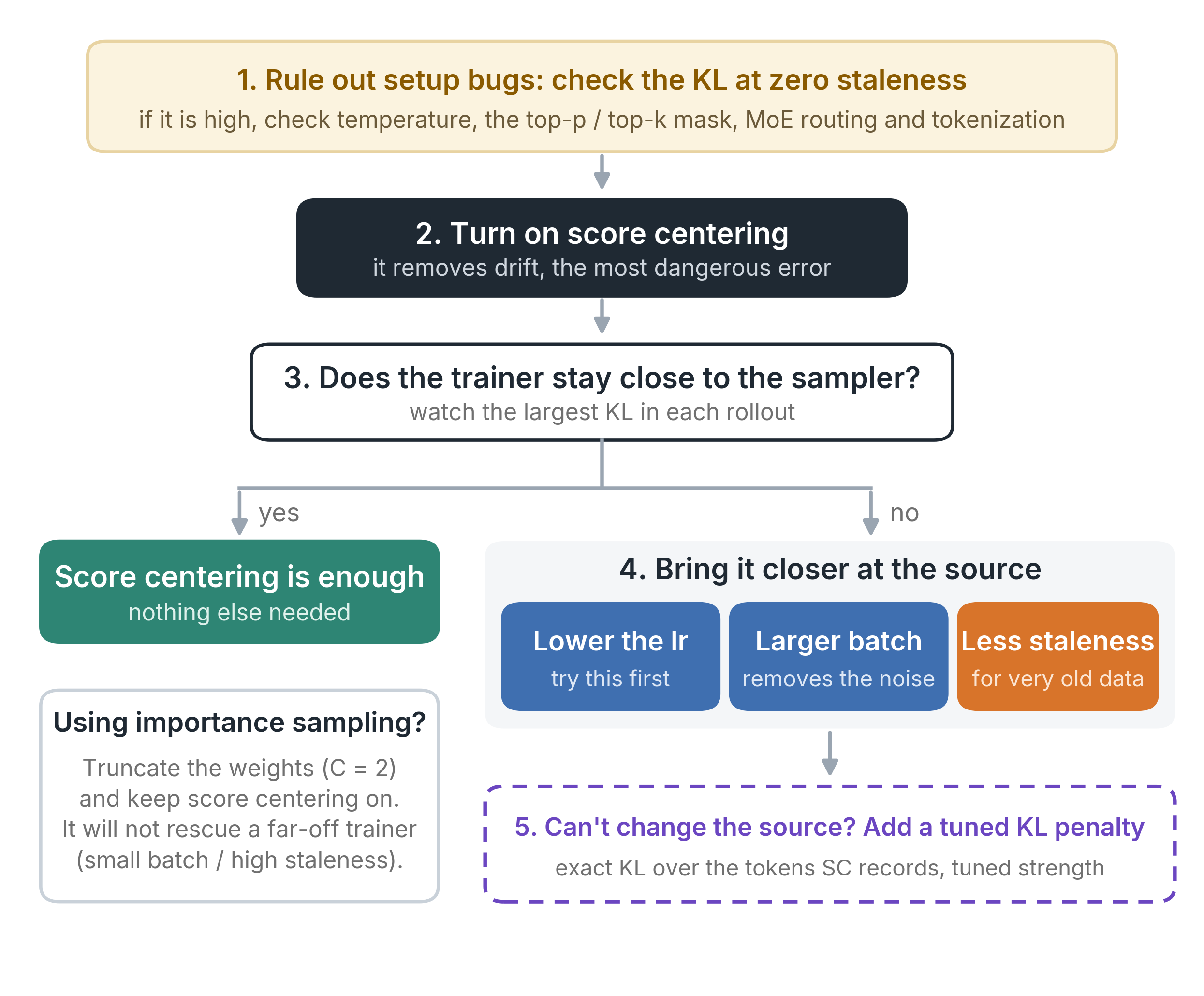
1. Rule out setup bugs. First measure the KL between the trainer and the sampler at zero staleness. It should be close to zero. If it is not, make sure the trainer uses the sampler’s temperature and top-p or top-k mask, replays its MoE routing, and trains on its token IDs instead of re-tokenized text, which can split differently. No correction can make up for a large mismatch from these bugs (Fang & Khazi, 2025).
2. Turn on score centering. Drift pushes every step in the same direction and grows on its own, so a larger batch cannot fix it, but score centering removes it. If you also use importance sampling, truncate the weights, since a single extreme weight can break vanilla IS.
3. Watch how far the trainer moves. The largest KL in each rollout is the signal to watch. While it stays small, score centering alone is enough.
4. If it grows, fix it at the source. Lower the learning rate first, since it matches the best KL penalty with nothing to tune. Use a larger batch while the distance is mostly noise, and reduce staleness when the data is very old.
5. Add a KL penalty only when the source cannot change, and tune its strength. Compute the exact KL over the tokens you already record for SC, not only the sampled one. The framework default strength can stop learning.
6. Conclusion
Score centering removes drift. What it leaves is distance, part noise and part learning itself, and this split explains why the two results we started from disagree. The SC paper trains with a large batch (i.e., 512 responses per step), which keeps the noise small and the trainer close to the sampler, so SC + TIS is stable. Zhang trains with a small batch (i.e., a few prompts per step) on data tens to hundreds of steps old, so the trainer moves far and SC + TIS collapses. Comparisons of off-policy corrections should therefore report batch size and staleness.
The split also points to what could come after SC. The levers it suggests need no new algorithm, because every RL run already has them. Once the batch is large enough to make the noise small, as in most large-scale training, the remaining distance comes mostly from learning on old data. This part grows with the learning rate times the staleness, so staler data calls for smaller steps. When async RL becomes unstable, it helps to first ask what broke it, whether noise, learning on old data, or a single extreme weight.
7. Open questions and related work
Several directions remain open, and they matter most for async RL at scale. Letting staleness follow the KL could keep training stable without giving up throughput. Testing Adam and Muon, which large runs use, would show whether the split between noise and learning still holds there. Understanding the sudden KL jumps at small batches, and comparing methods once each is tuned on its own, would make these recommendations more reliable.
Open questions
- Can staleness follow the KL instead of a fixed schedule? Async systems usually fix staleness in advance for throughput. In our runs, the largest KL in a rollout rises before SC collapses, and the last steps of a rollout add most of it. A sampler that syncs early only when this KL grows too large would give up throughput only when training needs it. How much throughput that costs, and which threshold to use, we have not tested.
- What triggers the sudden jump at small batches? Each SC + TIS collapse at small batches starts within a single rollout, where the largest KL goes from below 0.2 to between 3 and 33 together with a weight in the tens of thousands. We never see this at batch 512. Whether one rare token sets it off, or the trainer is already unstable before that weight appears, is still unclear.
- How much does SC add once every method is tuned? Every method in our runs used the same batch size and learning rate, and a method without SC might do better at other settings. Untruncated IS, for example, collapses at learning rate 0.03 at staleness 7 and batch 64, but trains to the end at 0.015. A fairer comparison would tune TIS and a KL penalty on their own, without SC, and compare each one’s best run with the best run of SC.
- Do the thresholds move under Adam or Muon? We use SGD so that a larger batch changes only the noise. Adam rescales every update, which ties the step size to the batch. Muon, which some large runs now use, orthogonalizes each update, so its step size depends less on the gradient’s scale. Whether the split between noise and learning survives under either optimizer, and where SC alone then stops being enough, remains to be seen.
Related work
Truncated importance sampling. Ionides (2008) introduces truncation with a ceiling \(\propto \sqrt{n}\). ACER and V-trace use fixed ceilings in deep RL. Yao et al. (2025) bring token-level TIS to LLM RL, and Liu et al. (2025) use it to train with 8-bit samplers. Later work finds that fixed ceilings mostly truncate low-confidence tokens (Yu et al., 2026) and that no single ceiling works throughout training (Zhou et al., 2026).
Score centering and KL penalties. Our drift decomposition follows Marek & Ryabinin (2026). Zhang (2026) bounds the error left by SC with the KL between the trainer and the sampler, observes that SC does not bound this KL, and adds a KL penalty that decays with staleness. To raise staleness, Zhang cuts each rollout into smaller steps, which also shrinks the batch, so the noise and signal terms grow together. Zhang’s SC + TIS also differs slightly from ours, but ours collapses at small batches too. Thinking Machines' StableReinforce uses REINFORCE + SC + a fixed-coefficient KL penalty (Marek, 2026). PRIME-RL’s IPO masks tokens whose probability difference exceeds a threshold, on both sides. In our framework, all of these limit the KL between the trainer and the sampler through the loss.
Trust regions. TRPO (Schulman et al., 2015) and PPO (Schulman et al., 2017) keep each update near the policy that collected the data, because the surrogate objective is only reliable there. We split that distance into a noise part and a signal part. A trust region, like a KL penalty, does not tell them apart.
Batch, noise, and KL. McCandlish et al. (2018) define the critical batch size via the gradient noise scale. Our two-term decomposition is its off-policy counterpart. Smith & Le (2018) describe SGD noise with a temperature \(\propto \eta/B\). The scaling rule matters. Linear scaling (Goyal et al., 2017) increases noise with the batch, while square-root scaling (Malladi et al., 2022) keeps it constant.
Acknowledgements
This project is built on top of SkyRL. The code is available in our GitHub repository. We thank Souradip Chakraborty, Daanish Khazi, Qiuyang Mang, Yi Pan, Charlie Ruan, Eric Tang, Yichuan Wang, Minghao Yan, and Chenxiao Yang for helpful discussions and feedback.
Citation
@misc{liu2026driftdistance,
  author       = {Liu, Shu and Fang, Qi and Agarwal, Shubham},
  title        = {Drift and Distance: When Is Score Centering Enough in Async RL?},
  howpublished = {Blog post},
  year         = {2026},
  url          = {https://rl-cookbook.github.io/sc-drift-and-distance/}
}
References
Espeholt, L., Soyer, H., Munos, R., et al. (2018). IMPALA: Scalable Distributed Deep-RL with Importance Weighted Actor-Learner Architectures. ICML 2018. arXiv:1802.01561
Goyal, P., Dollár, P., Girshick, R., et al. (2017). Accurate, Large Minibatch SGD: Training ImageNet in 1 Hour. arXiv:1706.02677
Ionides, E. L. (2008). Truncated Importance Sampling. Journal of Computational and Graphical Statistics. doi:10.1198/106186008X320456
Malladi, S., Lyu, K., Panigrahi, A., and Arora, S. (2022). On the SDEs and Scaling Rules for Adaptive Gradient Algorithms. NeurIPS 2022. arXiv:2205.10287
Marek, M. and Ryabinin, M. (2026). Score Centering Stabilizes Off-policy Reinforcement Learning. arXiv:2609.20807
McCandlish, S., Kaplan, J., Amodei, D., and OpenAI Dota Team (2018). An Empirical Model of Large-Batch Training. arXiv:1812.06162
PRIME-RL. IPO (INTELLECT Policy Optimization). PRIME-RL documentation. github.com/PrimeIntellect-ai/prime-rl/blob/main/docs/ipo.md
Smith, S. L. and Le, Q. V. (2018). A Bayesian Perspective on Generalization and Stochastic Gradient Descent. ICLR 2018. arXiv:1710.06451
Thinking Machines Lab. StableReinforce (alpha). Tinker documentation. tinker-docs.thinkingmachines.ai/tinker/losses/stable-reinforce
Wang, Z., Bapst, V., Heess, N., et al. (2017). Sample Efficient Actor-Critic with Experience Replay. ICLR 2017. arXiv:1611.01224
Yao, F., Liu, L., Zhang, D., Dong, C., Shang, J., and Gao, J. (2025). Your Efficient RL Framework Secretly Brings You Off-Policy RL Training. Blog post. fengyao.notion.site/off-policy-rl
Yu, T., Zhao, K., Li, S., et al. (2026). Rethinking Training-Inference Mismatch in LLM Reinforcement Learning: Where It Arises and How to Correct It. arXiv:2609.32444
Zhang, Y. (2026). Score Function Centering: Why a Stale Rollout Does Not Have to Be Importance Sampled. Blog post. normaluhr.github.io/en/p/score-function-centering-kl
Zhou, J., Shao, W., Zheng, L., et al. (2026). AIS: Adaptive Importance Sampling for Quantized RL. arXiv:2605.13907
Fang, Q., and Khazi, D. (2025). Mismatch Praxis: Rollout Settings and IS Corrections. Blog post. llmdata.com/blog/mismatch-praxis
Schulman, J., Levine, S., Moritz, P., Jordan, M. I., and Abbeel, P. (2015). Trust Region Policy Optimization. ICML 2015. arXiv:1502.05477
Schulman, J., Wolski, F., Dhariwal, P., Radford, A., and Klimov, O. (2017). Proximal Policy Optimization Algorithms. arXiv:1707.06347
Schulman, J. (2020). Approximating KL Divergence. Blog post. joschu.net/blog/kl-approx.html